Visualisization functions
Visualizing landscapes
We can use the plot function from terra
to have look at our landscape.
# Plot landscape
plot(landscape) 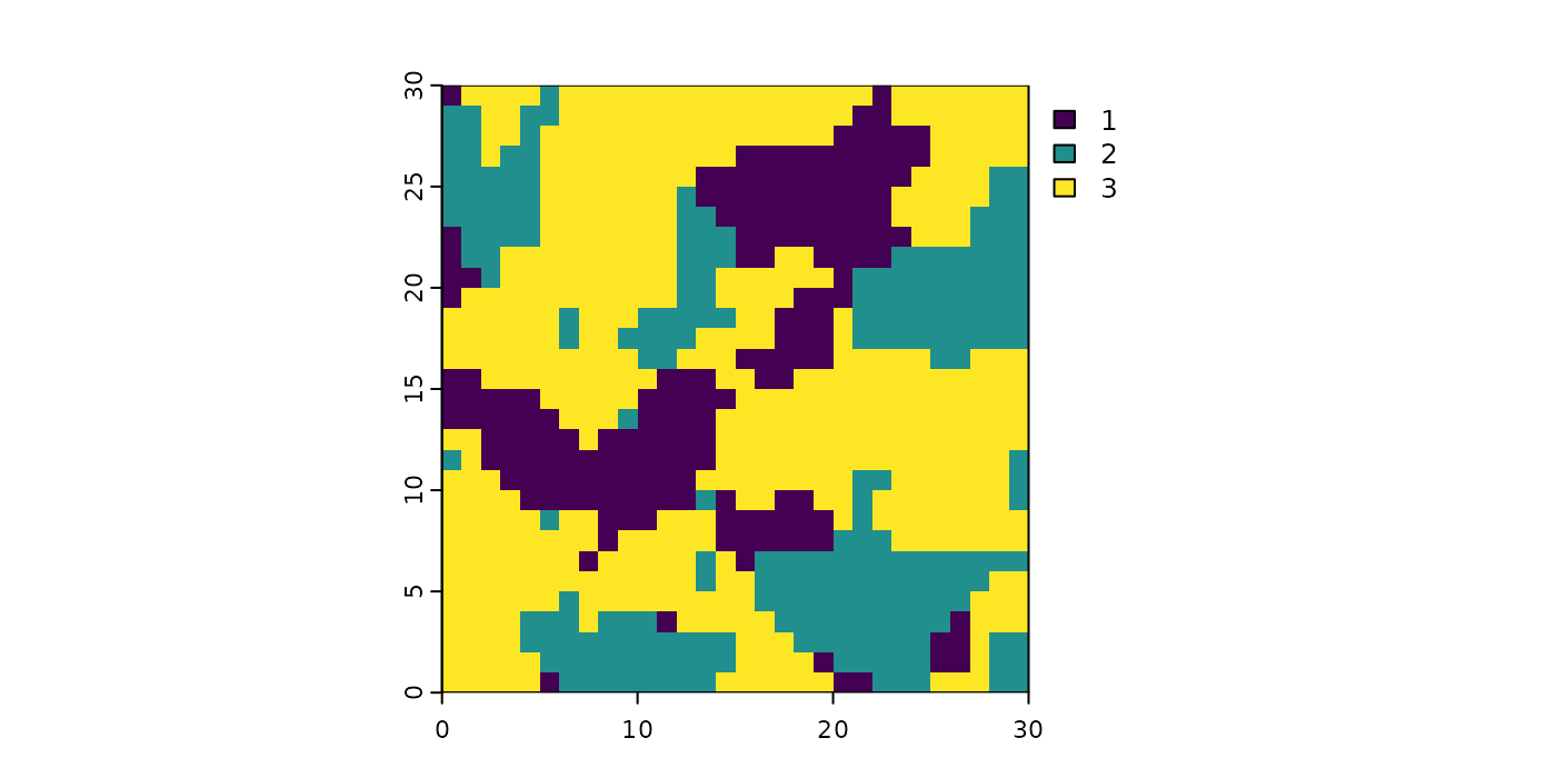
This is how we typically inspect our landscape, but which also makes it quite hard to relate to the landscape metrics we are interested in. This why we show in the following how to dissect this landscape visually into the components, that drive the calculation of landscape metrics.
Visualizing patches
To visualize patches in a landscape and encode each patch with an ID
that can be used to compare a landscape metric with the actual landscape
you can use the auxiliary visualisation function
show_patches():
# Plot landscape + landscape with labeled patches
show_patches(landscape)
#> $layer_1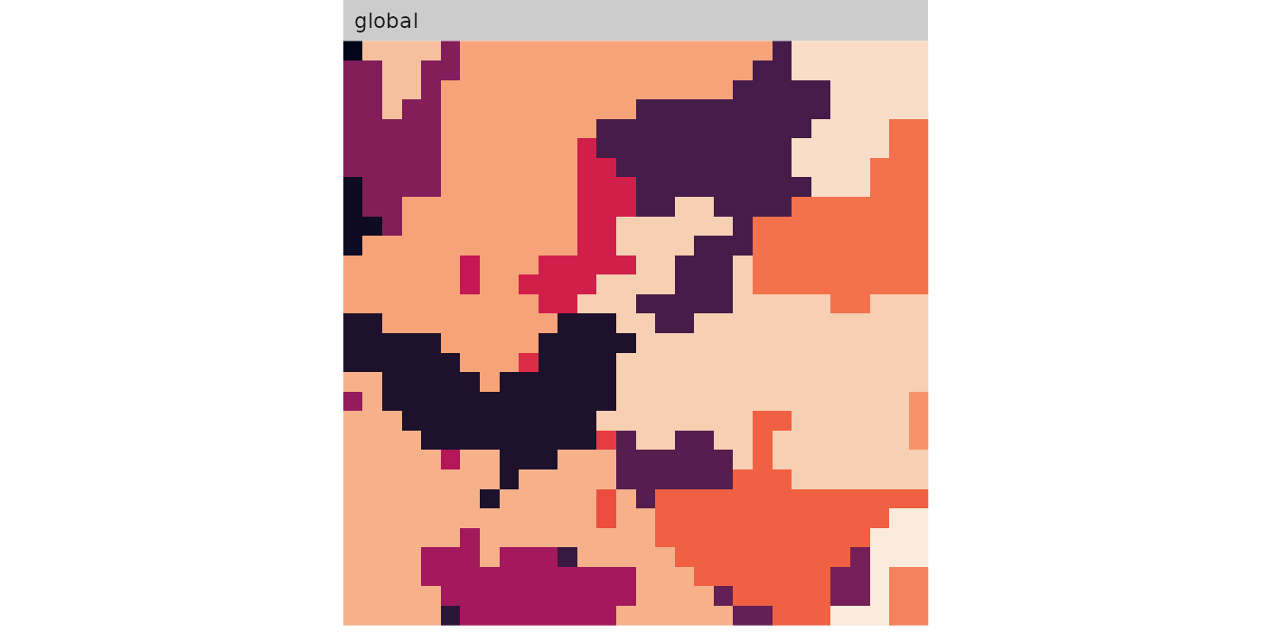
You can also plot all patches of each class grouped.
# show patches of all classes
show_patches(landscape, class = "all", labels = FALSE)
#> $layer_1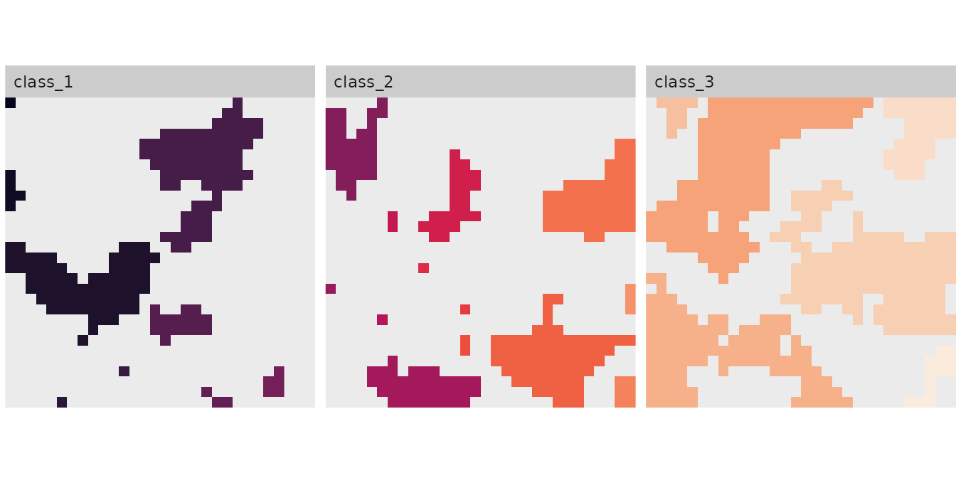
To show only the core area, there is the visualization function
show_cores. The arguments are similar to
show_patches():
# show core area of class 1 and 3
show_cores(landscape, class = c(1, 2), labels = FALSE)
#> $layer_1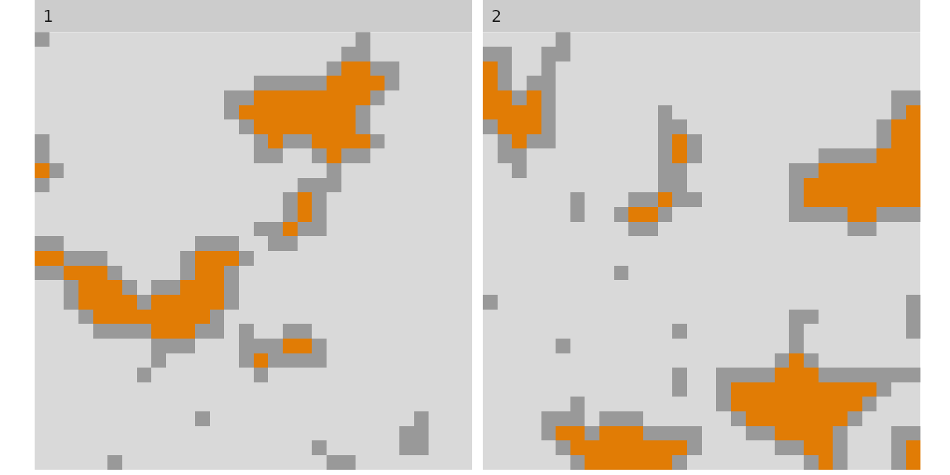
Lastly, you can also “fill” the colours of each patch according to
its value of a certain patch level metric, e.g., the patch area, using
show_lsm(). You can chose if the label should be the patch
id or the actual value of the landscape metric
(label_lsm = TRUE/FALSE).
# fill patch according to area
show_lsm(landscape, what = "lsm_p_area", class = "global", label_lsm = TRUE)
#> $layer_1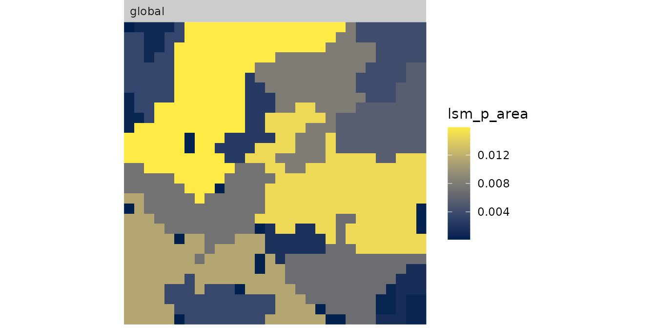
To get the result as a SpatRaster, there is
spatialize_lsm().
spatialize_lsm(landscape, what = "lsm_p_area")
#> Warning: Please use 'check_landscape()' to ensure the input data is valid.
#> $layer_1
#> $layer_1$lsm_p_area
#> class       : SpatRaster
#> dimensions  : 30, 30, 1  (nrow, ncol, nlyr)
#> resolution  : 1, 1  (x, y)
#> extent      : 0, 30, 0, 30  (xmin, xmax, ymin, ymax)
#> coord. ref. :
#> source(s)   : memory
#> name        :  value
#> min value   : 0.0001
#> max value   : 0.0159
Show correlation
Selecting meaningful landscape metrics for your field of research is difficult, as many landscape metrics are very abstract and the common approach is often simply to calculate as many as possible.
To select at the least that ones for your landscape and research
question that are not highly correlated, you can use the function
show_correlation() to get a first insight into the
correlation of the metrics you calculated:
metrics <- calculate_lsm(landscape, what = "patch")
#> Warning: Please use 'check_landscape()' to ensure the input data is valid.
show_correlation(metrics, method = "pearson")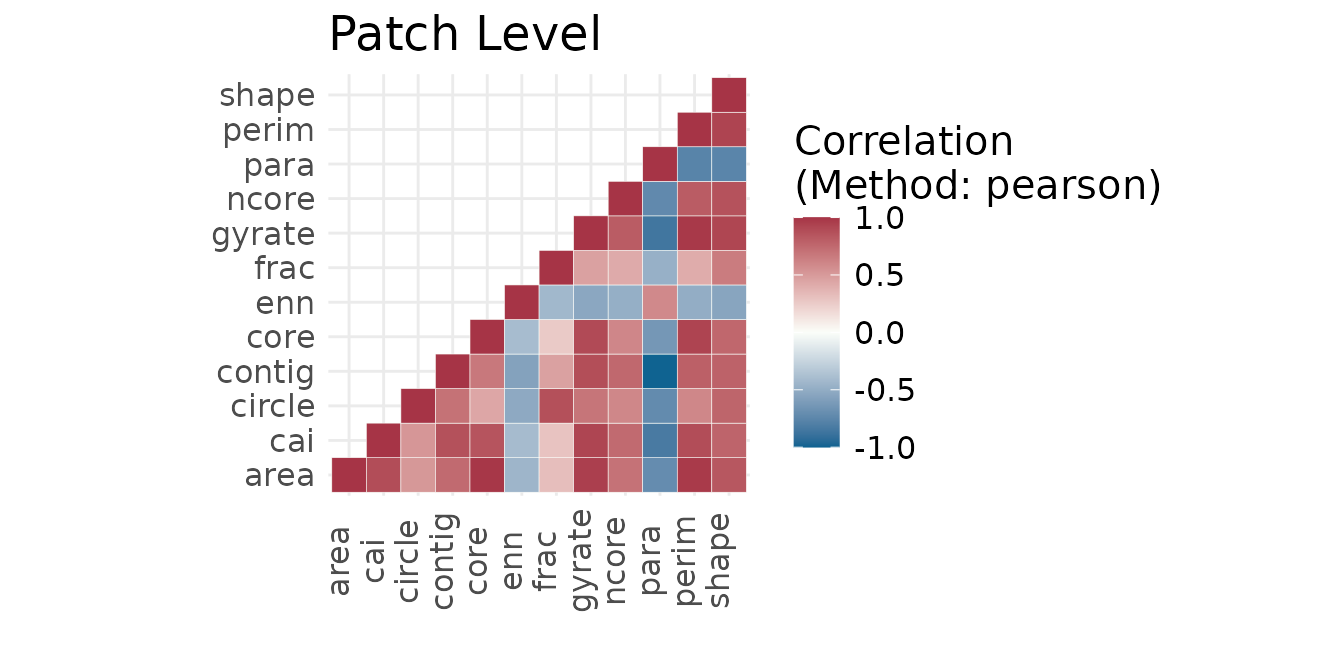
Building blocks
Get patches
landscapemetrics makes internally heavy use of an
connected labeling algorithm and exports an re-implementation of this
algorithm (get_patches()). This function return a list,
where each list entry includes all patches of the corresponding class.
The patches are labeled from 1…to n.
# get a list of all patches for each class
get_patches(landscape)
#> $layer_1
#> $layer_1$class_1
#> class       : SpatRaster
#> dimensions  : 30, 30, 1  (nrow, ncol, nlyr)
#> resolution  : 1, 1  (x, y)
#> extent      : 0, 30, 0, 30  (xmin, xmax, ymin, ymax)
#> coord. ref. :
#> source(s)   : memory
#> name        : lyr.1
#> min value   :     1
#> max value   :     9
#>
#> $layer_1$class_2
#> class       : SpatRaster
#> dimensions  : 30, 30, 1  (nrow, ncol, nlyr)
#> resolution  : 1, 1  (x, y)
#> extent      : 0, 30, 0, 30  (xmin, xmax, ymin, ymax)
#> coord. ref. :
#> source(s)   : memory
#> name        : lyr.1
#> min value   :    10
#> max value   :    22
#>
#> $layer_1$class_3
#> class       : SpatRaster
#> dimensions  : 30, 30, 1  (nrow, ncol, nlyr)
#> resolution  : 1, 1  (x, y)
#> extent      : 0, 30, 0, 30  (xmin, xmax, ymin, ymax)
#> coord. ref. :
#> source(s)   : memory
#> name        : lyr.1
#> min value   :    23
#> max value   :    28
Get adjacencies
Adjacencies are a central part for landscape metrics, so calculating them quick and in a flexible way is key for, e.g., developing new metrics. Hence, landscapemetrics exports a function that can calculate adjacencies in any number if directions when provided with a binary matrix (NA / 1 - NA are cells that would be left out for looking at adjacencies).
# calculate full adjacency matrix
get_adjacencies(landscape, neighbourhood = 4)
#> $layer_1
#>     1   2    3
#> 1 542  44  137
#> 2  44 696  159
#> 3 137 159 1562

# count diagonal neighbour adjacencies
diagonal_matrix <- matrix(c(1,  NA,  1,
                            NA,  0, NA,
                            1,  NA,  1), 3, 3, byrow = TRUE)
get_adjacencies(landscape, diagonal_matrix)
#> $layer_1
#>     1   2    3
#> 1 486  56  169
#> 2  56 592  215
#> 3 169 215 1406

# equivalent with the terra package:
adj_terra <- function(x){
    adjacencies <- terra::adjacent(x, 1:terra::ncell(x), "rook", pairs=TRUE)
    table(terra::values(x, mat = FALSE)[adjacencies[,1]],
          terra::values(x, mat = FALSE)[adjacencies[,2]])
}

# compare the two implementations
bench::mark(
    get_adjacencies(landscape, neighbourhood = 4),
    adj_terra(landscape),
    iterations = 250,
    check = FALSE
)
#> # A tibble: 2 × 6
#>   expression                             min median `itr/sec` mem_alloc `gc/sec`
#>   <bch:expr>                          <bch:> <bch:>     <dbl> <bch:byt>    <dbl>
#> 1 get_adjacencies(landscape, neighbo… 2.31ms 2.56ms      386.    22.6KB    16.1
#> 2 adj_terra(landscape)                3.33ms 3.67ms      268.   874.1KB     5.47

adj_terra(landscape) == get_adjacencies(landscape, 4)[[1]]
#>
#>        1    2    3
#>   1 TRUE TRUE TRUE
#>   2 TRUE TRUE TRUE
#>   3 TRUE TRUE TRUE
Get nearest neighbour
landscapemetrics implements a memory efficient and quite fast way to calculate the nearest neighbour between classes in a raster (or matrix).
# run connected labeling for raster
patches <- get_patches(landscape, class = 1)

# calculate the minimum distance between patches in a landscape
min_dist <- get_nearestneighbour(patches$layer_1$class_1)

# create a function that would do the same with the raster package
nn_terra <- function(patches) {

    np_class <- terra::values(patches[[1]][[1]]) |>
        na.omit() |>
        unique() |>
        length()

    points_class <- terra::as.data.frame(patches[[1]][[1]], xy = TRUE)

    minimum_distance <- seq_len(np_class) |>
        purrr::map_dbl(function(patch_ij) {

            patch_focal <- dplyr::filter(points_class, lyr.1 == patch_ij) |>
                dplyr::select(x, y) |>
                as.matrix(ncol = 2)

            patch_others <- dplyr::filter(points_class, lyr.1 != patch_ij) |>
                dplyr::select(x, y) |>
                as.matrix(ncol = 2)

            minimum_distance <- terra::distance(patch_focal, patch_others,
                                                lonlat = FALSE) |>
                min()
        })

    data.frame(id = unique(sort(points_class$lyr.1)), distance = minimum_distance)

}


# compare the two implementations
bench::mark(
    get_nearestneighbour(patches$layer_1$class_1)[, 2:3],
    nn_terra(patches$layer_1$class_1),
    iterations = 250, check = FALSE
)
#> # A tibble: 2 × 6
#>   expression                             min median `itr/sec` mem_alloc `gc/sec`
#>   <bch:expr>                         <bch:t> <bch:>     <dbl> <bch:byt>    <dbl>
#> 1 get_nearestneighbour(patches$laye…  4.61ms  4.9ms     202.   283.89KB     4.97
#> 2 nn_terra(patches$layer_1$class_1)  43.59ms 46.5ms      21.3    2.83MB     6.88

# check if results are identical
get_nearestneighbour(patches$layer_1$class_1)[, 2:3] == nn_terra(patches$layer_1$class_1)
#>         id dist
#>  [1,] TRUE TRUE
#>  [2,] TRUE TRUE
#>  [3,] TRUE TRUE
#>  [4,] TRUE TRUE
#>  [5,] TRUE TRUE
#>  [6,] TRUE TRUE
#>  [7,] TRUE TRUE
#>  [8,] TRUE TRUE
#>  [9,] TRUE TRUE
Get circumscribing circle
To get the smallest circumscribing circle that includes all cells of
the patch, simply run get_circumscribingcircle(). The
result returns the diameter for each circle that includes all cells of
each patch. This includes not only the cell centers but the whole cells
using the cells corners.
# get all patches of class 1
class_1 <- get_patches(landscape, class = 1)

# get smallest circumscribing circle for each patch
circle <- get_circumscribingcircle(class_1$layer_1$class_1)
circle
#> # A tibble: 9 × 7
#>   layer level class    id value center_x center_y
#>   <int> <chr> <int> <int> <dbl>    <dbl>    <dbl>
#> 1     1 patch     1     1  1.41     0.5      29.5
#> 2     1 patch     2     2  4.12     0.5      21
#> 3     1 patch     3     3 15.5      7.38     13.7
#> 4     1 patch     4     4  1.41     5.5       0.5
#> 5     1 patch     5     5  1.41    11.5       3.5
#> 6     1 patch     6     6 16.6     19.5      22.5
#> 7     1 patch     7     7  6.71    17         8.5
#> 8     1 patch     8     8  3.61    20.5       1
#> 9     1 patch     9     9  3.61    26         2.5