General background
2025-02-11
Source:vignettes/articles/general_background.Rmd
general_background.RmdIntroduction
Ecology and landscape ecology mainly studies interactions between organisms and their environment. In a wider sense, the environment perceived by the organism can be defined as a landscape. This can spread from huge areas for, e.g., mobile, large-bodied mammals to much smaller areas for, e.g., immobile insects and always depends on the research question.
Landscape metrics are tools to characterize a landscape. This includes mainly describing the composition and configuration of a landscape. While the composition basically describes how much of the landscape is occupied by a certain land cover type, the configuration mainly describes the spatial arrangement of the land cover types. The basic idea of landscape metrics is to condense as much information as possible into single number.
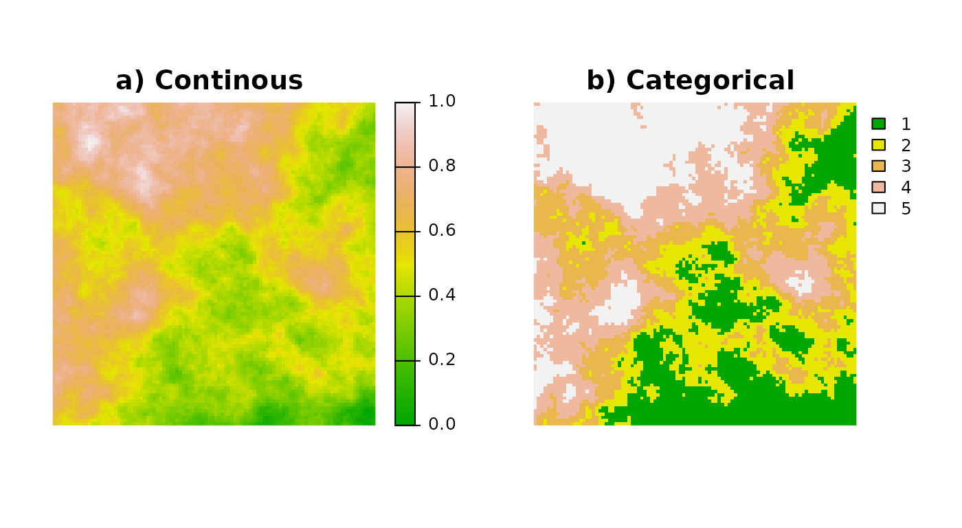
The landscapemetrics package supports terra spatial objects. A raster (sometimes also referred to as grid) contains spatial information by dividing the landscape into discrete cells. Consequently, the cells are the smallest “resolution of information”. Because landscapemetrics deals with categorical data, each cell has to be assigned to a discrete class (see Fig. 1 for details). These classes must be positive integer numbers.

Fig 1.: a) and b) are the same landscape, but with a continous (a) and categorical (b) representation. A continuous landscape would typically be expected from remote sensing imagery or interpolated enviromental data. Categorical landscapes are mostly classified as percieved by humans, e.g. in land cover and use classes.
Levels of landscape metrics
Landscape metrics can be calculated for three different levels (or “scales”). Each level contains information about different aspects of the landscape. Level of interest depends largely on the research question, and often a combination of several levels can be useful. Similar, also the decision of which metric to use depends on the research question asked.
A patch is defined as neighboring cells belonging to
the same class i. Hereby, landscapemetrics
uses the 8-neighbors rule (Queen’s case) to identify patches. Patch
level metrics are calculated for every patch in the landscape,
regardless of the class that the patch belongs to. The output will match
the number of patches present in the landscape. These metrics are also
often the basis for metrics of the other two levels.
Class level metrics summaries all patches belonging
to one class i. These metrics can be either the
“distribution” of patch level metrics of all patches of class
i (e.g., the mean) or consider only patches of class
i for the calculations of the metric. Regardless of the
mathematical background, the output will always match the number of
classes present. Class level metrics are suitable to describe the
composition and configuration of the landscape.
Landscape level metrics summaries the whole landscape into one value. This can either be done by summarising metrics of lower levels or calculating a metric including all patches and classes. Following, the output will always be just one number. Landscape level metrics are suitable for condensing information about the landscape into just one value.
Classes of landscape metrics
There are six different classes of landscape metrics implemented in landscapemetrics:
Area and edge metrics describe the size of patches and classes and the amount of edge. An edge is defined as the border between two patches of class
iandkin meters. These metrics mainly characterize the composition of the landscape and are able to show dominance or rareness of classes.Shape metrics describe the shape of patches, mainly by using its area and perimeter. This can be important for many research questions, because, e.g., even though, being equal in size, long and narrow patches have probably different characteristics than a squared patch of the same size.
Core metrics describe the area of patches that are not an edge. These metrics can be interesting for research questions in which, e.g., only areas that are not influenced by neighboring patches of a different class are of interest.
Aggregation metrics describe if patches (of the same class) are rather clumped (aggregated) or tend to be isolated. Following, these metrics describe mainly the spatial configuration of the landscape.
Diversity metrics are only available on the landscape level. They describe the abundance and dominance/rareness of classes. Thereby, they show the diversity of present classes.
Complexity metrics For more information, please see New Metrics outside FRAGSTATS.
Other software to calculate landscape metrics
There are already software packages available to calculate landscape
metrics, the most famous one probably being the stand-alone software
FRAGSTATS (McGarigal et al. 2023). But also add-ons to GIS
software are available, e.g. r.le (Baker & Cai 1992) or its
successor r.li for GRASS GIS. Lastly, also an R package, namely
SDMTools (VanDerWal et al. 2014), can be used.
Nevertheless, we decided to re-implement most of the metrics
available in FRAGSTATS.
We wanted to provide a comprehensive collection of landscape metrics in
R. While FRAGSTATS is an extensive collection it is only available for
Windows. Note, that even though we tried to re-implement the metrics as
described in the FRAGSTATS manual, there are some differences (Differences
FRAGSTATS|landscapemetrics). Further, SDMTools contains
only a subset of metrics and does not cover all levels (General
background). Lastly, we want to start a collection of landscape
metrics being open source and easily extendable by new (future)
landscape metrics (see CONTRIBUTING).
Also, one major advantage of landscapemetrics are the
utility functions for, e.g., the visualization or sampling of landscape
metrics.
Those were the main reasons we implemented landscapemetrics, however, we want to fully appreciate and acknowledge the already present software.
References
- Baker, W.L. and Cai, Y. 1992. The r.le programs for multiscale analysis of landscape structure using the GRASS geographical information system. Landscape Ecology 7(4):291-302.
- McGarigal K., SA Cushman, and E Ene. 2023. FRAGSTATS v4: Spatial Pattern Analysis Program for Categorical Maps. Computer software program produced by the authors; available at the following web site: https://www.fragstats.org
- VanDerWal, J., Falconi, L., Januchowski, S., Shoo, L., and Storlie, C. 2014. SDMTools: Species Distribution Modelling Tools: Tools for processing data associated with species distribution modelling exercises. R package version 1.1-221. https://CRAN.R-project.org/package=SDMTools