Sampling around points of interest

2024-04-02

library(landscapemetrics)
library(terra)
library(sf)
library(ggplot2)

# internal data needs to be read
landscape <- terra::rast(landscapemetrics::landscape)

landscapemetrics provides several functions to sample metrics at or around sample points. On possible application for this feature could be a study in which the study organism only encounters the landscape within a local neighborhood of sample points. For most functions, sample points can be provided as a 2-column matrix(x- and y-coordinate), or sf objects (Pebesma 2018) are supported.

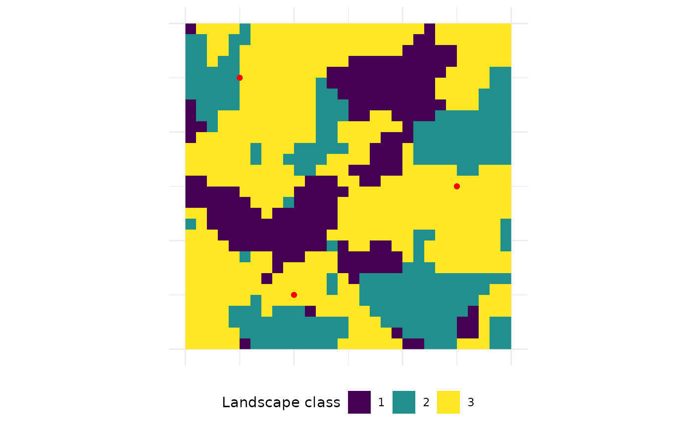
First, we create some example sample locations.

# create some example points
(points <- matrix(c(10, 5, 25, 15, 5, 25), ncol = 2, byrow = TRUE))
##      [,1] [,2]
## [1,]   10    5
## [2,]   25   15
## [3,]    5   25

# # create some example lines
# x1 <- c(1, 5, 15, 10)
# y1 <- c(1, 5, 15, 25)
# x2 <- c(10, 25)
# y2 <- c(5, 5)
# 
# sample_lines <- sf::st_multilinestring(x = list(cbind(x1, y1), cbind(x2, y2)))

Extract landscape metrics at sample points

extract_lsm() returns the metrics of all patches in which a sample point is located. However, since this only makes sense for individual patches, it’s only possible to extract patch-level metrics.

Now, it’s straightforward to extract e.g. the patch area of all patches in which a sample point is located. Similar to all functions calculating several landscape metrics, the selected metrics can be specified by various arguments (see list_lsm() for more details). The resulting tibble includes one extra column (compared to calculate_lsm()), indicating the ID of the sample points.

Because three sample points were provided and only the patch area was requested, the resulting tibble also has three rows - one for each sample point. The first and the second sample point are actually located in the same patch and following also the area is identical. The third sample point is located in a much smaller patch. The tibble gives also information about the patch ids and the land-cover classes in which sample points are located.

extract_lsm(landscape, y = points, what = "lsm_p_area")
## Warning: Please use 'check_landscape()' to ensure the input data is valid.
## # A tibble: 3 × 7
##   layer level class    id metric  value extract_id
##   <int> <chr> <int> <int> <chr>   <dbl>      <int>
## 1     1 patch     3    24 area   0.0113          1
## 2     1 patch     3    26 area   0.0148          2
## 3     1 patch     3    23 area   0.0159          3

Sample landscape metrics at sample points

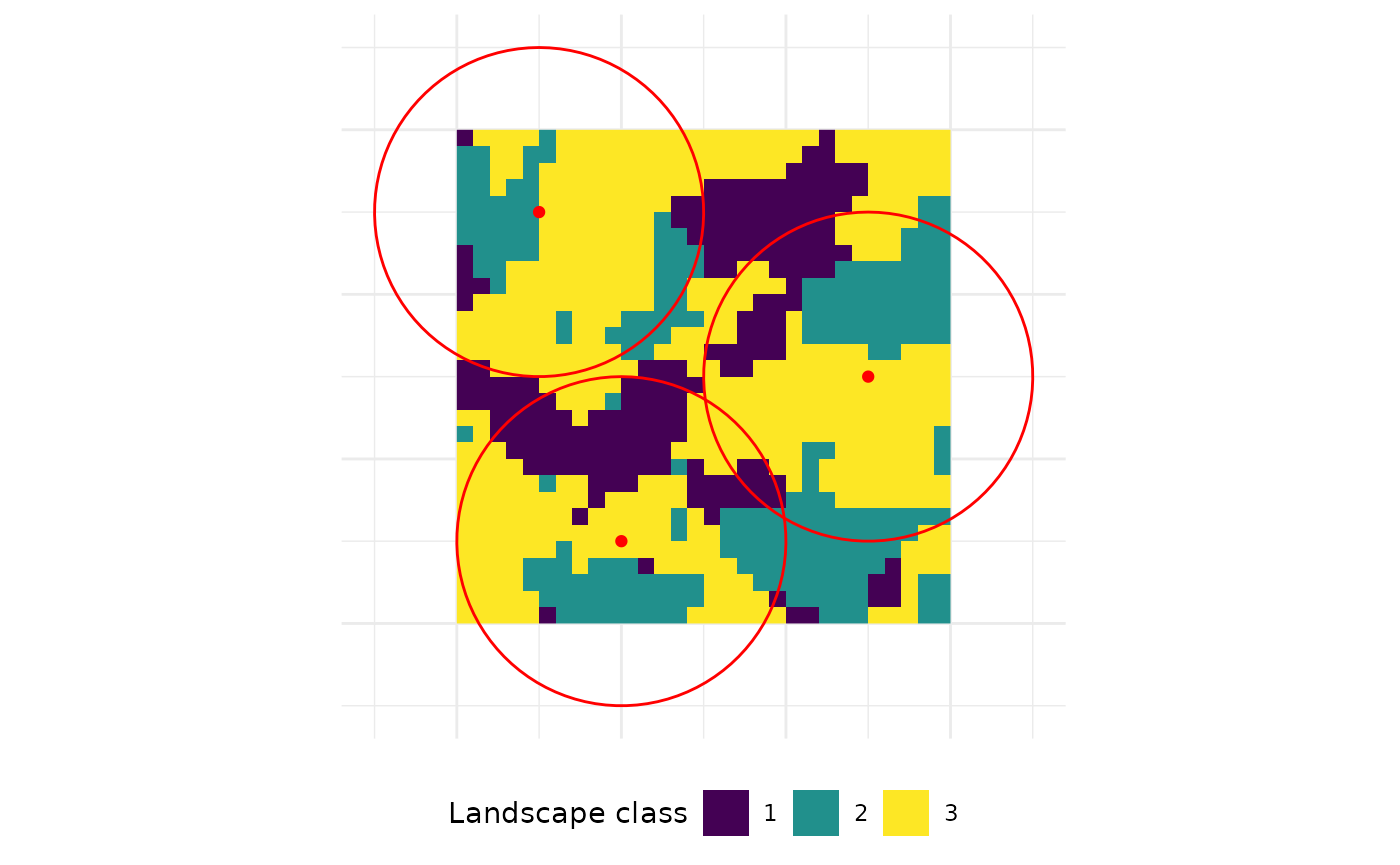
To sample landscape metrics within a certain buffer around sample points, there is sample_lsm(). Now, the size of the buffers around the sample locations must be specified. The functions clips the landscape within the buffer (in other words sample plots) and calculates the selected metrics.

The resulting tibble includes two extra columns. Again, the id of the sample point is included. Furthermore, the size of the actual sampled landscape can be different to the provided size due to two reasons. Firstly, because clipping raster cells using a circle or a sample plot not directly at a cell center lead to inaccuracies. Secondly, sample plots can exceed the landscape boundary. Therefore, we report the actual clipped sample plot area relative in relation to the theoretical, maximum sample plot area e.g. a sample plot only half within the landscape will have a percentage_inside = 50.

sample_lsm(landscape, y = points, size = 10, 
           level = "landscape", type = "diversity metric", 
           classes_max = 3, verbose = FALSE)
## # A tibble: 27 × 8
##    layer level     class    id metric     value plot_id percentage_inside
##    <int> <chr>     <int> <int> <chr>      <dbl>   <int>             <dbl>
##  1     1 landscape    NA    NA msidi      0.947       1                75
##  2     1 landscape    NA    NA msiei      0.862       1                75
##  3     1 landscape    NA    NA pr         3           1                75
##  4     1 landscape    NA    NA prd    10000           1                75
##  5     1 landscape    NA    NA rpr      100           1                75
##  6     1 landscape    NA    NA shdi       1.02        1                75
##  7     1 landscape    NA    NA shei       0.928       1                75
##  8     1 landscape    NA    NA sidi       0.612       1                75
##  9     1 landscape    NA    NA siei       0.918       1                75
## 10     1 landscape    NA    NA msidi      0.969       2                75
## # ℹ 17 more rows

References

Pebesma, E., 2018. Simple Features for R: Standardized Support for Spatial Vector Data. The R Journal, https://journal.r-project.org/archive/2018/RJ-2018-009/

Roger S. Bivand, Edzer Pebesma, Virgilio Gomez-Rubio, 2013. Applied spatial data analysis with R, Second edition. Springer, NY. http://www.asdar-book.org/