Calculating landscape metrics for irregular areas

Landscape metrics are quantitative measures that describe the composition and configuration of a landscape. In this vignette, we will use the R package landscapemetrics to calculate landscape metrics for irregular areas.

To get started, we first need to install and attach the required R packages. We will use landscapemetrics, sf, terra, and tidyr in this example:

library(landscapemetrics)
library(sf)
library(terra)
library(tidyr)

Next, we need to read in our example data. In this case, we will use the Augusta NLCD dataset and an example set of irregular polygons provided by the landscapemetrics package:

# read example data ----------------------------------------------------
augusta_nlcd = rast(landscapemetrics::augusta_nlcd)
irregular_areas <- landscapemetrics:::internal_data$irregular_areas

plot(augusta_nlcd, type = "classes")
plot(st_geometry(irregular_areas), add = TRUE)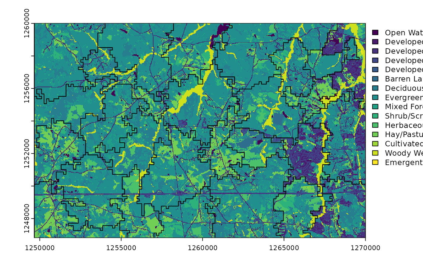

In the code above, we read in the Augusta NLCD dataset as a raster object and the example irregular polygons as an sf object. We then plot both of these objects together to visualize our data.

We can calculate landscape metrics for the whole landscape using the calculate_lsm() function:

# calculate lsm for the whole landscape -----------------------------------
all_landscape = calculate_lsm(augusta_nlcd, what = c("lsm_l_ent", "lsm_l_condent", 
                                                      "lsm_l_mutinf", "lsm_l_joinent", 
                                                      "lsm_l_relmutinf"))

all_landscape

## # A tibble: 5 × 6
##   layer level     class    id metric    value
##   <int> <chr>     <int> <int> <chr>     <dbl>
## 1     1 landscape    NA    NA condent   1.63 
## 2     1 landscape    NA    NA ent       2.88 
## 3     1 landscape    NA    NA joinent   4.51 
## 4     1 landscape    NA    NA mutinf    1.24 
## 5     1 landscape    NA    NA relmutinf 0.432

Here, we specify the what argument to calculate a set of landscape metrics that include entropy, conditional entropy, mutual information, joint entropy, and relative mutual information. We store the calculated landscape metrics in the all_landscape object.

On the other hand, we can also calculate landscape metrics for irregular polygons using the sample_lsm() function:

# calculate lsm for irregular polygons ------------------------------------
irr_landscapes = sample_lsm(augusta_nlcd, irregular_areas,
                            what = c("lsm_l_ent", "lsm_l_condent",
                                     "lsm_l_mutinf", "lsm_l_joinent", 
                                     "lsm_l_relmutinf"))

irr_landscapes

## # A tibble: 135 × 8
##    layer level     class    id metric    value plot_id percentage_inside
##    <int> <chr>     <int> <int> <chr>     <dbl>   <int>             <dbl>
##  1     1 landscape    NA    NA condent   1.17        1              102.
##  2     1 landscape    NA    NA ent       1.93        1              102.
##  3     1 landscape    NA    NA joinent   3.10        1              102.
##  4     1 landscape    NA    NA mutinf    0.757       1              102.
##  5     1 landscape    NA    NA relmutinf 0.393       1              102.
##  6     1 landscape    NA    NA condent   1.19        2              105.
##  7     1 landscape    NA    NA ent       2.18        2              105.
##  8     1 landscape    NA    NA joinent   3.37        2              105.
##  9     1 landscape    NA    NA mutinf    0.984       2              105.
## 10     1 landscape    NA    NA relmutinf 0.452       2              105.
## # ℹ 125 more rows

Here, we use the sample_lsm() function to calculate the same set of landscape metrics for our example set of irregular polygons. We store the results in the irr_landscapes object.

We can connect the calculated landscape metric values to our original polygons using the pivot_wider() function:

# connect values to polygons ----------------------------------------------
irr_landscapes_w = pivot_wider(irr_landscapes, 
                               id_cols = plot_id,
                               names_from = metric, 
                               values_from = value)

irregular_areas = cbind(irregular_areas, irr_landscapes_w)

Here, we pivot the irr_landscapes object from a long format to a wide format using the pivot_wider() function. We specify the id_cols, names_from, and values_from arguments to connect the calculated landscape metric values to our original polygons. We then add the calculated landscape metrics as columns to our original irregular_areas object using cbind().

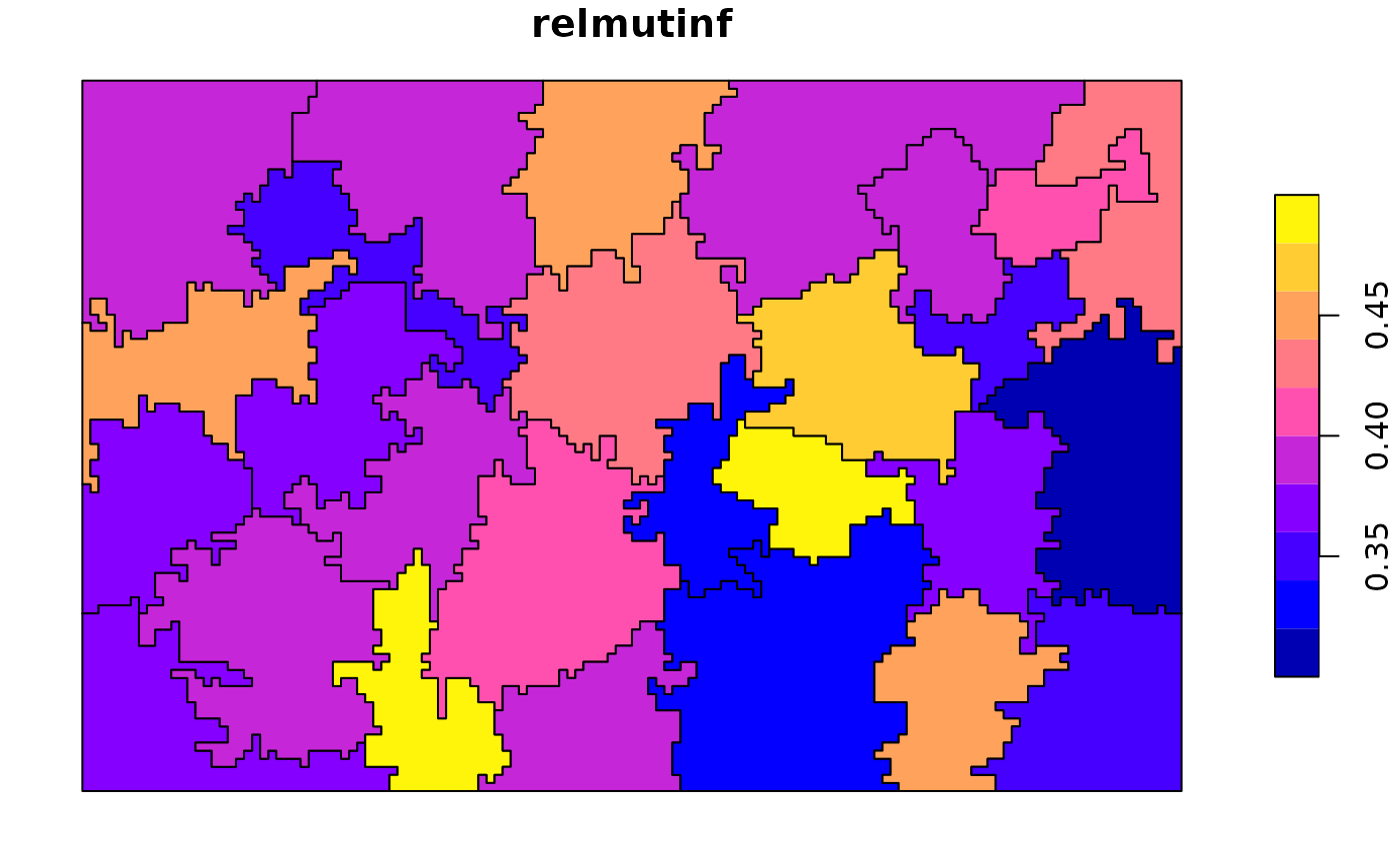
Finally, we can visualize the calculated landscape metrics using the plot() function:

# viz results -------------------------------------------------------------
plot(irregular_areas["ent"])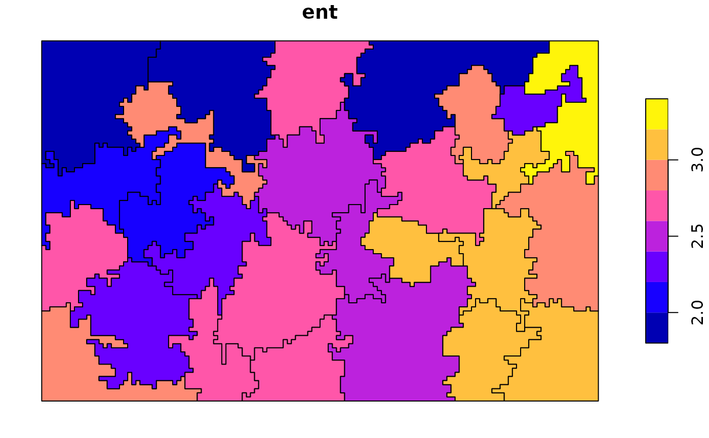

plot(irregular_areas["condent"])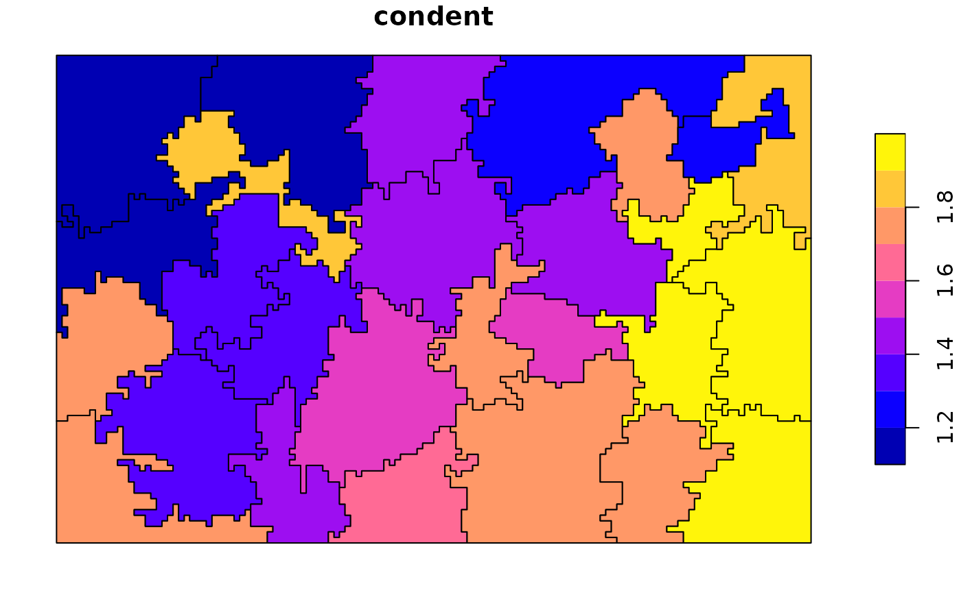

plot(irregular_areas["mutinf"])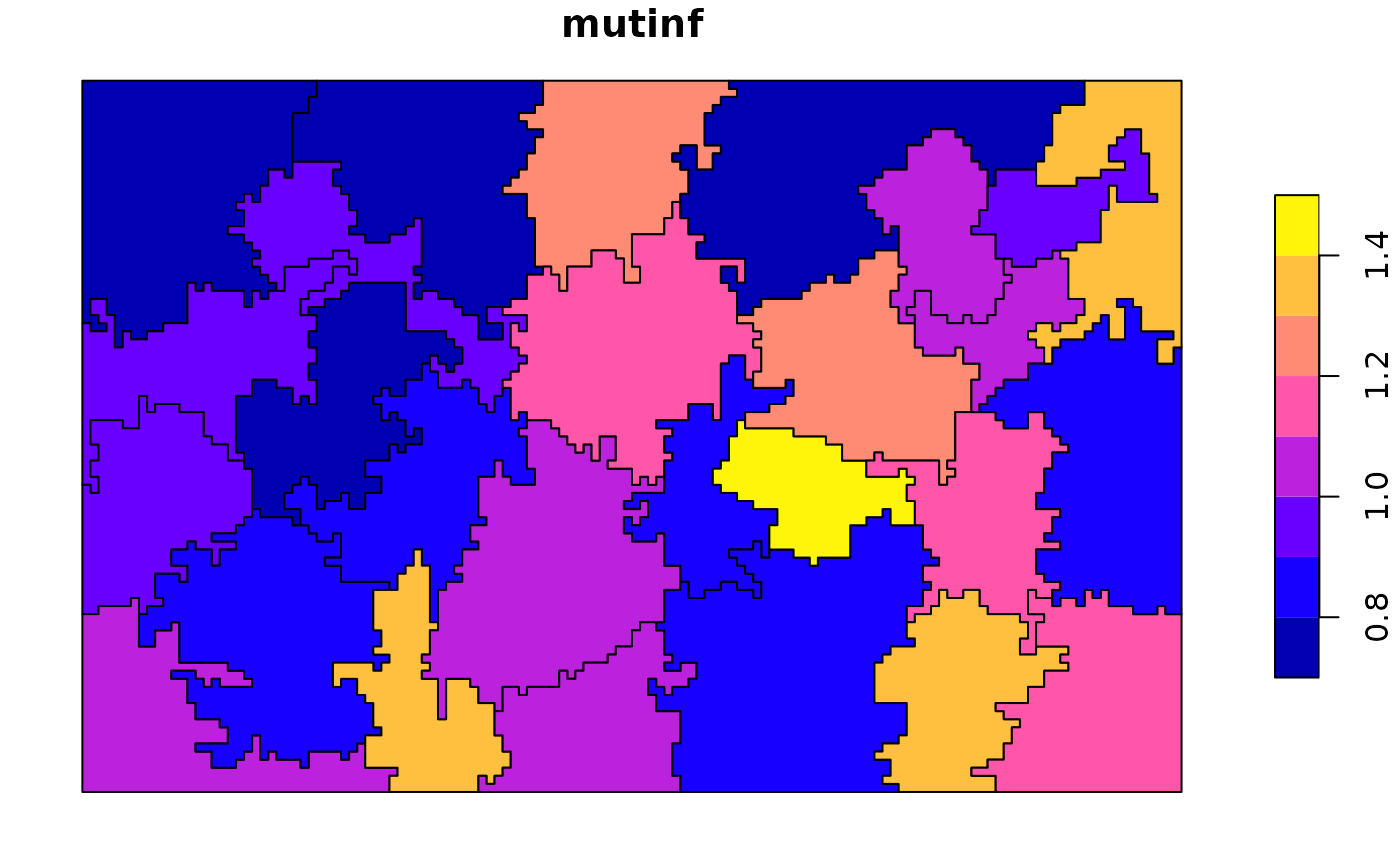

plot(irregular_areas["joinent"])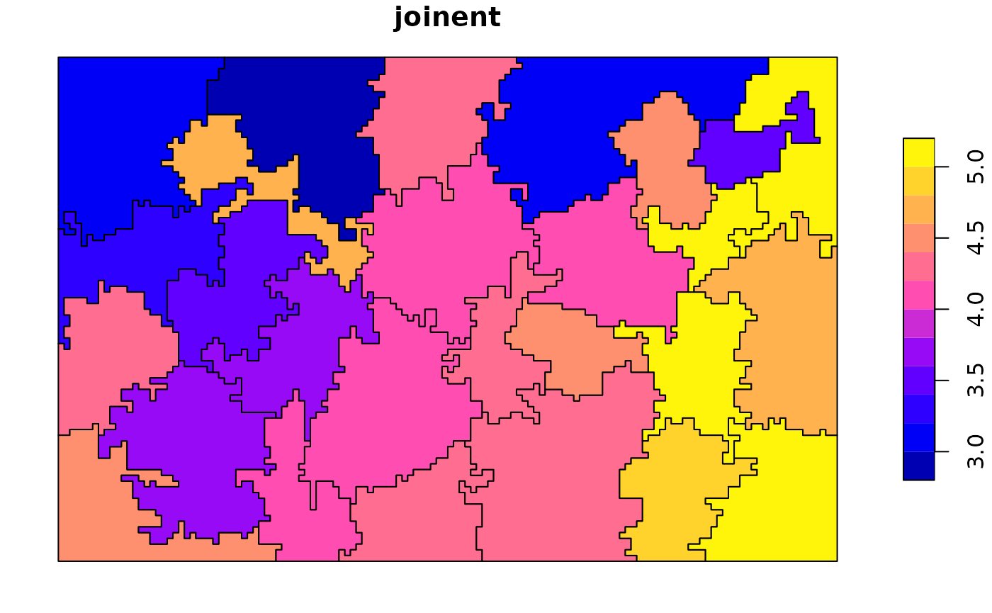

plot(irregular_areas["relmutinf"])

2024-04-02