Analysing the climatic niche of Cormus domestica

Outline

This vignette demonstrates how to use shar to analyse species occurrence data obtained from the Global Biodiversity Information Facility (GBIF) and environmental raster data obtained from the Climate Research Unit (CRU) entirely in R. The “Gamma test” approach as detailed in the vignette("background") is used. The distribution of the tree species Cormus domestica in Europe is selected, a tree which tolerates a wide range of conditions but favors warm to mild climates, occurring in the “Subtropical dry forest” and “Temperate Continental” FAO ecological zones. Cormus domestica is most commonly found in Southern Europe, though there it’s natural range is uncertain owing to it’s cultivation and distribution by the Roman Empire (De Rigo et al., 2016; Rotach, 2003).

Load required packages

This article of the package requires the getCRUCLdata package, which is not available on CRAN anymore. To install the package, please run install.packages('getCRUCLdata', repos = 'http://packages.ropensci.org', typ = 'source').

library(dplyr) # For data wrangling
library(getCRUCLdata) # For retrieving climate raster data
library(ggplot2) # For plotting
library(patchwork) # For composing multiple plots
library(rgbif) # For retrieving species occurrence data
library(rnaturalearth) # For retrieving geographical data
library(rnaturalearthdata) # For retrieving geographical data
library(sf) # For spatial data operations
library(spatstat) # For spatial point pattern analysis
library(terra) # For spatial data operations
library(shar) # For species-habitat association analysis

Download occurrence data

To retrieve species occurrence data the R package rgbif (Chamberlain & Boettiger, 2017) is used, which provides an interface to access the GBIF database. For this vignette we are interested in observations within the likely natural distribution of Cormus domestica, which includes Europe, the wider Mediterranean, the Black Sea Region, and potentially North Africa.

# Retrieve key for Cormus domestica
key <- rgbif::name_backbone(name = 'Cormus domestica', kingdom = 'plants')

# Establish region of interest
roi <- c(xmin = -20, xmax = 45, ymin = 30, ymax = 73)
roi_bbox <- sf::st_bbox(roi, crs = sf::st_crs("EPSG:4326"))
roi_sfc <- sf::st_sfc(sf::st_point(c(roi[["xmin"]], roi[["ymin"]])), 
                      sf::st_point(c(roi[["xmax"]], roi[["ymax"]])), 
                      crs = "EPSG:4326")

# Retrieve occurrences for the region of interest
res <- rgbif::occ_search(taxonKey = as.numeric(key$usageKey), limit = 99999, 
                         geometry = roi_bbox)

# Create a simple data frame containing only the unique identifier (id),
# latitude (lat), and longtitude (lon).
data_simp <- data.frame(id = res$data$key, 
                        lat = res$data$decimalLatitude, lon = res$data$decimalLongitude) %>% 
  dplyr::filter(!is.na(lat) | !is.na(lon))

Download map data

Spatial polygon data for the world is obtained from the rnaturalearth package (South, 2022), the map is then restricted to the region of interest. The spatstat package requires geospatial data in the format of a projected coordinate system; the data is therefore converted from the geographic coordinate system 4336 to the projected coordinate system 3395. The shar function fit_point_process requires a spatial point pattern (ppp) object bounded within an observation window of the class owin, which is then created.

# Retrieve data from rnaturalearth
worldmap <- rnaturalearth::ne_countries(returnclass = "sf", scale = 50) %>%
  sf::st_transform(crs = sf::st_crs("EPSG:3395"))

# Re-project simple features region of interest
roi_sfc_3395 <- roi_sfc %>%
  sf::st_transform(crs = sf::st_crs("EPSG:3395"))

# Crop world map to include polygons within the region of interest
roi_map <- sf::st_crop(x = worldmap, y = roi_sfc_3395)

# Define observation window
roi_owin <- spatstat.geom::as.owin(roi_map$geometry)

Download climate data

The environmental variable selected for demonstrative purposes is the mean temperature in January over the 1961-1990 period. Data is obtained through the getCRUCLdata package (Sparks, 2017) which provides access to the datasets described in New et al. (2002).

# Download data as a raster brick through the getCRUCLdata package
# Mean temperature (tmn) data should be 180.4MB
cru_data <- getCRUCLdata::get_CRU_stack(tmp = TRUE)

# Select temperature variable and the month of January
tmp_raster <- cru_data$tmp$jan

Prepare landscape raster

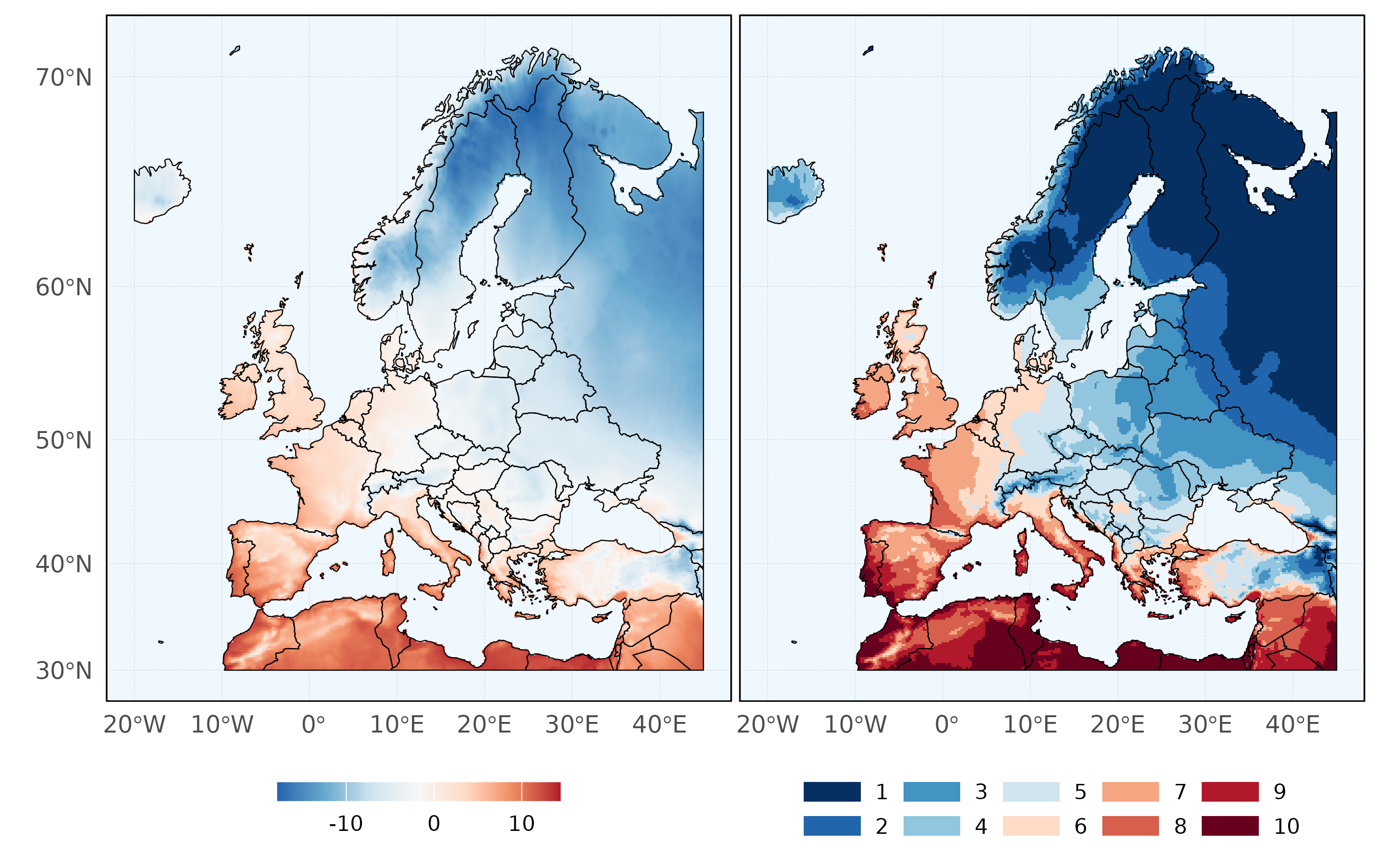
The climate data obtained above is restricted to the region of interest, then classified into 10 habitats based on temperature ranges, achieved by setting the lower and upper bounds of these ranges in the fixedBreaks argument of the classify_habitats function. Figure 1 displays the unclassified and classified habitat.

# Crop tmp raster
tmp_raster_eur <- terra::crop(x = tmp_raster, y = roi)

# Project raster to EPSG:3395
tmp_raster_eur_3395 <- terra::project(x = tmp_raster_eur, y = "EPSG:3395", 
                                      method = "bilinear")

# Classify landscape
landscape_classified <- shar::classify_habitats(raster = tmp_raster_eur_3395,
                                                return_breaks = TRUE, style = "fixed",
                                                fixedBreaks = c(-20, -10, -7.5, -5, -2.5, 
                                                                0, 2.5, 5, 7.5, 10, 20))

Figure 1 - The mean temperature in January over the 1961-1990 period on a continuous scale (left) and classified in to ten discrete categories (right).

Prepare occurrence data

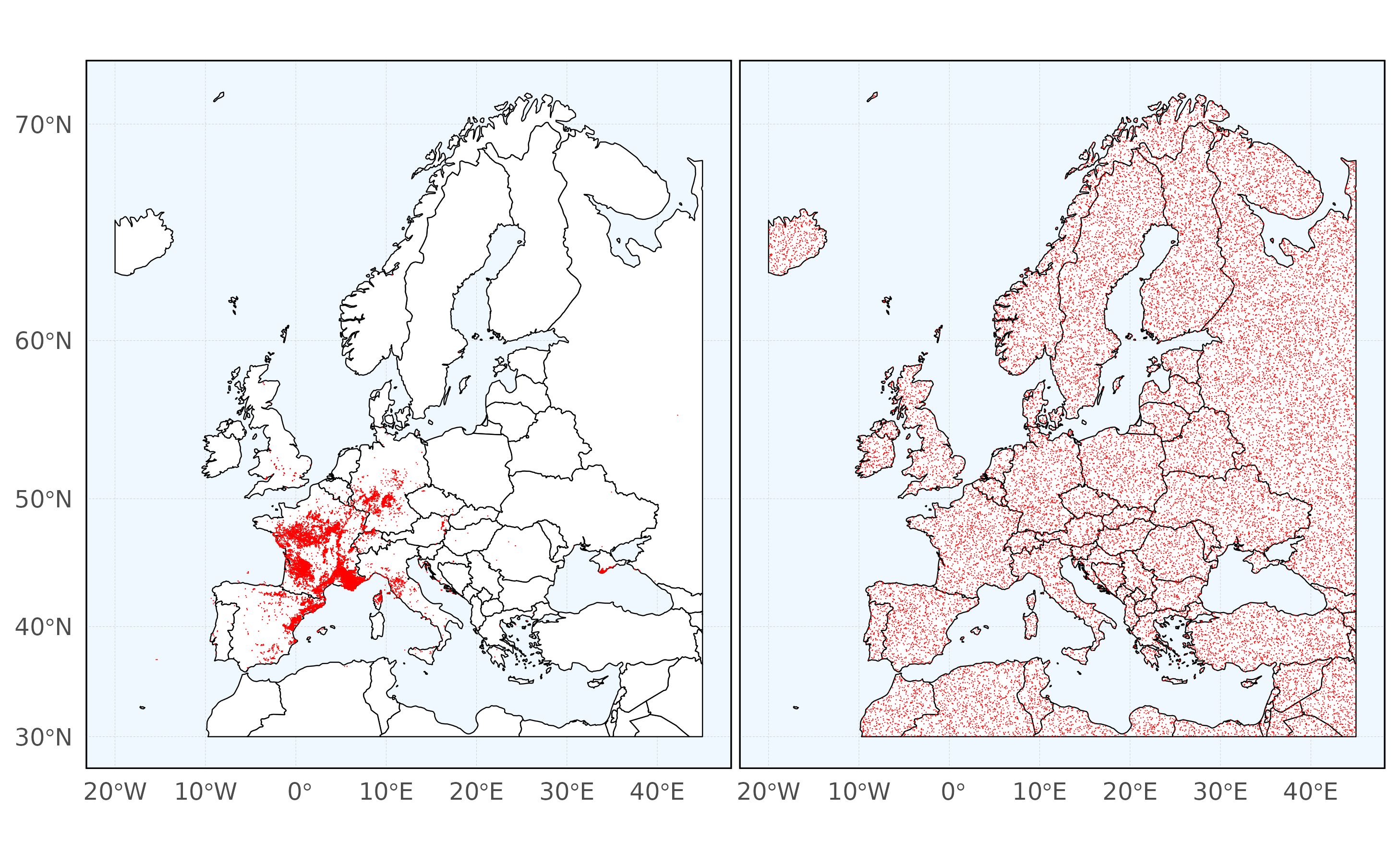
The occurrence data is prepared, then the shar function fit_point_process is called, yielding the randomized occurrence data within the observation window as required by the results_habitat_association function. Figure 2 displays the real and randomised occurrence data.

# Convert occurrence data to a simple features object
data_sf <- sf::st_as_sf(data_simp, coords = c("lon", "lat"), crs = "EPSG:4326")

# Re-project the occurrence data
data_sf_3395 <- data_sf %>%
  sf::st_transform(crs = sf::st_crs("EPSG:3395"))

# Extract the coordinates as a matrix from the sf occurrences object
data_sf_coords <- sf::st_coordinates(data_sf_3395)

# Create a spatial points pattern object containing the occurrence data
data_sf_ppp <- spatstat.geom::as.ppp(X = data_sf_coords, W = roi_owin)

# Fit point pattern process to data
rand_pattern <- shar::fit_point_process(pattern = data_sf_ppp, n_random = 19)

Figure 2 - Real (left) and randomised (right) occurrences of Cormus domestica.

Results

The analysis function results_habitat_association is then called. The results of the analysis show that Cormus domestica is positively associated with locations which experience a mean January temperature of -2.5C - 10C (habitats 5, 6, 7, 8, and 9). Furthermore, Cormus domestica is negatively associated with all other habitats classified by temperature.

# Establish significance level
sig_level <- 0.01

# Run analysis
results <- shar::results_habitat_association(pattern = rand_pattern, 
                                             raster = landscape_classified$raster,
                                             breaks = landscape_classified$breaks,
                                             significance_level = sig_level) %>% 
  dplyr::arrange(habitat)

results
#>    habitat     breaks count      lo      hi significance
#> 1        1  [-20,-10)     1 8897.81 9178.68     negative
#> 2        2 [-10,-7.5)     0 2928.76 3144.28     negative
#> 3        3  [-7.5,-5)    11 3283.53 3381.46     negative
#> 4        4  [-5,-2.5)   162 3185.54 3392.96     negative
#> 5        5   [-2.5,0)  3744 2665.72 2908.96     positive
#> 6        6    [0,2.5)  5703 1791.80 1936.57     positive
#> 7        7    [2.5,5) 11802 2004.45 2147.30     positive
#> 8        8    [5,7.5)  7102 1646.23 1863.58     positive
#> 9        9   [7.5,10)  1719 1369.72 1511.67     positive
#> 10      10    [10,20)    57 1617.70 1768.31     negative

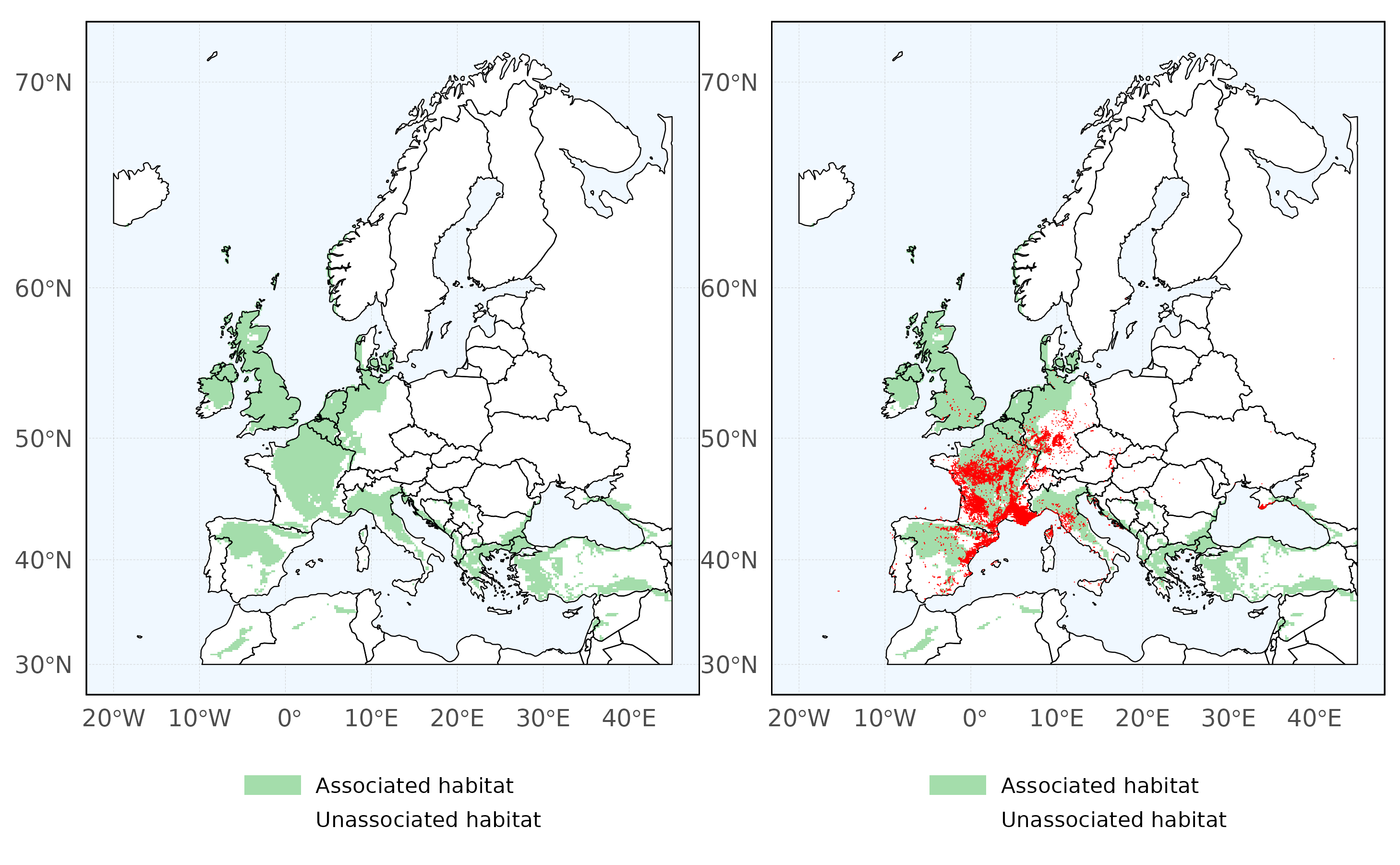
Figure 3 - The climatic niche of Cormus domestica, as defined by a positive association with a mean January temperature of -2.5C - 10C

By visually inspecting Figure 3 we can see that occurrences of Cormus domestica are mostly restricted to the associated habitat as defined by a mean January temperature of -2.5C - 10C. However, Cormus domestica does not exist in all areas experiencing a mean January temperature of -2.5C - 10C, additionally there are a number of occurrences outside these areas. The next step assessing in the climatic niche of Cormus domestica would be to repeat the above analysis for more environmental variables, which is beyond the scope of this minimal example.

References

Chamberlain SA, Boettiger C. 2017. R Python, and Ruby clients for GBIF species occurrence data. PeerJ Preprints 5:e3304v1 doi:10.7287/peerj.preprints.3304v1

De Rigo, D., Caudullo, G., Houston Durrant, T. and San-Miguel-Ayanz, J., 2016. The European Atlas of Forest Tree Species: modelling, data and information on forest tree species. European Atlas of Forest Tree Species, p.e01aa69. doi:10.2788/4251

New, M., Lister, D., Hulme, M. and Makin, I., 2002. A high-resolution data set of surface climate over global land areas. Climate research, 21(1), pp.1-25. doi:10.3354/cr021001

Rotach, P., 2003. EUFORGEN Technical Guidelines for genetic conservation and use for service tree (Sorbus domestica). Bioversity International.

South A (2022). rnaturalearth: World Map Data from Natural Earth. https://docs.ropensci.org/rnaturalearth (website) https://github.com/ropensci/rnaturalearth.

Sparks, (2017). getCRUCLdata: Use and Explore CRU CL v. 2.0 Climatology Elements in R. Journal of Open Source Software, 2(12), 230, doi:10.21105/joss.00230

Zeke Marshall

2024-12-17